Orders, lines and waves
Timestamped demand, SKU velocity, order size, cutoff logic, cancellations and replenishment.
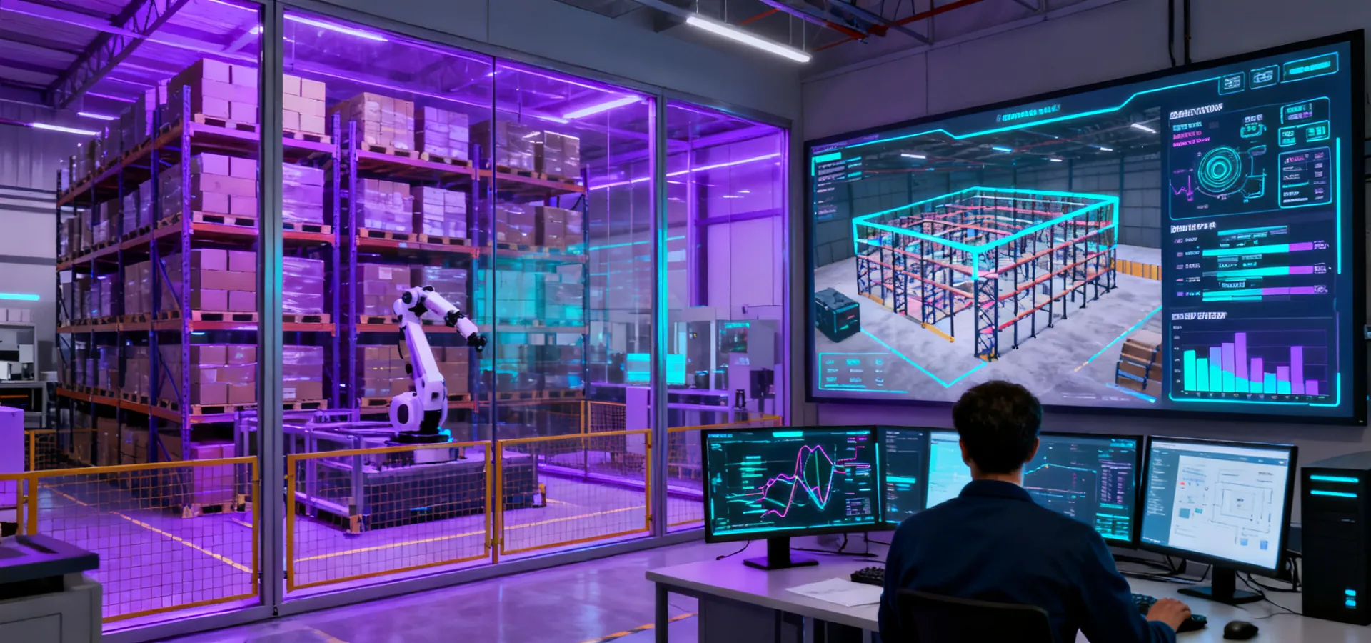
Expose throughput assumptions, storage density trade-offs, interface behavior and recovery paths before the live warehouse becomes the test environment. Models remain useful only when their inputs, simplifications and acceptance links are visible.
Inspect the input contractThe input contract names source, period, owner, unit and treatment for each dataset. Order history is separated from forecast scenarios. Physical travel distance is separated from nominal speed. Failure and recovery assumptions are listed beside the responsible control layer.
Missing information is not silently replaced by a favorable default. It is marked as an assumption with a sensitivity test, an owner and a date for confirmation. This makes later design changes traceable instead of turning the model into an unreviewable black box.
Timestamped demand, SKU velocity, order size, cutoff logic, cancellations and replenishment.
Rated load, center of gravity, aisle clear width, rack geometry, floor condition and station envelope.
Priorities, batching, charging, blocked destinations, retry limits and manual interventions.
WMS, WCS, WES, PLC and robot messages, interface cycle time, confirmations, timeouts and ownership.
Every reported output carries the scenario identifier, input revision and warm-up or observation period. A result is interpreted inside that boundary rather than promoted as a universal system rate.
Tests normal SKU and order distributions, replenishment, breaks and routine station variability. The baseline checks whether queues and storage retrievals are stable before peak or failure cases are introduced.
Raises release demand for the defined duration while retaining realistic downstream capacity. This distinguishes a brief burst from a system that holds stable output throughout the shipping cutoff.
Removes a route, robot, crane lane or transfer point and applies the agreed control response. The run shows whether failure remains isolated and how much time is required to clear accumulated work.
Emulated devices respond to commands, delay confirmations and inject defined faults so interface behavior can be reviewed ahead of site commissioning. The method is useful for message structure and state transitions; it cannot prove wireless coverage, physical sensor performance or real load stability.
A documented responsibility matrix identifies which layer detects each condition, which layer decides the next state and who authorizes a restart. Tests cover normal transfer, duplicate message, delayed response, invalid identity, loss of communication and controlled recovery.
A requirement identifier links the operating need, model scenario, interface or physical test, result and open issue. The trace prevents a simulated result from being mistaken for a completed site test.
State the rate, density or response with operating boundary and owner.
Identify the input revision, model build, event set and output definition.
Record emulated interfaces, expected states, observed log and deviation status.
Repeat applicable checks with installed geometry, real loads and site systems.
Higher cube utilization may reduce direct access, fire-protection flexibility and recovery options unless aisles and maintenance paths are designed explicitly.
More buffer, alternate routing and safe recovery may lower the clean-run maximum while improving stable output during disturbance.
Start with a representative order file, load-unit table, scaled layout, shift calendar, process logic and interface list. Mark forecast assumptions and the acceptance questions the model must answer.